Understanding the ROC Curve

• Why Is It Called "Receiver Operating Characteristic"?
• Interpreting the Curve
• What Does "Random Guessing" Actually Mean?
• Conclusion

The ROC curve is one of the most common ways to evaluate a binary classifier, but its name — Receiver Operating Characteristic — doesn't tell you anything about what it actually measures. Digging into where the name comes from turns out to be a useful way into understanding the curve itself, and the "random guessing" baseline that's usually drawn on it is a lot more precise than the standard hand-wave explanation suggests.

Why Is It Called "Receiver Operating Characteristic"?

The phrase sounds like overengineered academic jargon, but it's actually a historical relic. It wasn't coined by computer scientists — it came from British radar operators in World War II, who needed a way to describe how well they could tell a real enemy aircraft apart from birds or static on their screens.

Each word in the phrase maps directly onto both the original radar setup and the machine learning workflow that later borrowed it:

• Receiver — Then: the operator and radar equipment trying to distinguish a real aircraft from birds or clouds. Now: your binary classifier trying to distinguish a target class (e.g., spam) from background noise (e.g., normal email).
• Operating — Then: turning the sensitivity dial to filter out static or rain. Now: sliding the decision threshold — e.g., moving the classification cutoff from 0.5 to 0.7 — to change how aggressively the model guesses "positive."
• Characteristic — Then: the resulting graph of planes detected versus false alarms at each dial setting. Now: the curve itself — the trade-off between the True Positive Rate and the False Positive Rate across every possible threshold.

So the "Receiver Operating Characteristic" was originally just: how well a radar operator performs as their equipment is tuned. Translated into modern terms, it's a model's performance profile as its decision threshold is swept from one extreme to the other.

The stakes that shaped this trade-off were real. During the 1941 Blitz, British radar operators had to decide in real time whether a blip on the screen was a bomber or a flock of birds. Too sensitive, and they triggered false air raid sirens that caused mass panic and halted factory production. Not sensitive enough, and bombs fell without warning. The curves they plotted were a tool for finding the best dial setting given that trade-off. Psychologists picked up the same technique in the 1950s to study human perception, and it eventually made its way into machine learning as a way to evaluate classifiers — the name just never got updated.

Interpreting the Curve

An ROC curve plots two rates against each other:

Every point on the curve corresponds to one specific decision threshold. At a threshold of 1.0, the model never predicts "positive," so both FPR and TPR are 0 — that's the bottom-left corner, $(0, 0)$. As you lower the threshold, the model starts calling more cases positive: it catches more true positives (TPR climbs), but it also starts misfiring on negatives (FPR climbs too). At a threshold of 0.0, the model calls everything positive, landing on the top-right corner, $(1, 1)$. The ROC curve is just this sweep, plotted as one continuous line from $(0,0)$ to $(1,1)$.

Below is an ROC curve for a classifier with an AUC (area under the curve) of 0.98, with the point corresponding to the default threshold of 0.5 marked in red:

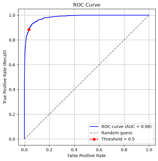
A few things to read off a curve like this:

• The closer the curve hugs the top-left corner, the better. That corner is $(FPR=0, TPR=1)$ — catching every true positive while triggering zero false alarms.
• The diagonal from $(0,0)$ to $(1,1)$ is the "no-skill" baseline. It represents a classifier whose predictions carry no real information about the true label. Any curve that bows up and to the left of it is doing better than that baseline; a curve below it is doing worse.
• AUC condenses the whole curve into one number — the probability that the model ranks a randomly chosen positive example above a randomly chosen negative one. An AUC of 0.5 means no better than the diagonal; 1.0 means perfect separation.

That diagonal baseline is usually described as "random guessing," which raises a natural question: what does random guessing actually mean here, precisely?

What Does "Random Guessing" Actually Mean?

It's common to hear that the $y=x$ line on an ROC curve represents random guessing, but that phrase glosses over a real subtlety. "Random guessing" could mean a few different things — flip a coin and guess positive or negative with equal probability, or always guess the majority class. Those don't sound equivalent, and under class imbalance the second one can even look like it performs well. So why do they all land on the same diagonal line?

The precise definition. A point on the ROC curve is $(FPR, TPR)$ at some threshold. The diagonal comes from a specific family of classifiers: ones whose predicted label is generated independently of the true label — the model doesn't look at the features, or its output simply carries no information correlated with $y$.

Formally, suppose the classifier outputs "positive" with some probability $p$, independent of the true class. Then:

Both equal $p$ — regardless of the actual class distribution — because $p$ doesn't depend on $y$ at all. As $p$ sweeps from 0 to 1, it traces out every point on the line $TPR = FPR$, i.e. the diagonal. The coin-flip case is the clearest instance: $p=0.5$ gives $TPR=0.5$, $FPR=0.5$, landing on the point $(0.5, 0.5)$ — squarely on the diagonal, matching intuition.

The "always guess the majority class" case is where it gets interesting. Say the data is 90% negative, 10% positive, and the model always predicts negative ($p=0$ for "positive"):

• $TPR = P(\text{predict positive} \mid \text{actual positive}) = 0$
• $FPR = P(\text{predict positive} \mid \text{actual negative}) = 0$

That's the point $(0, 0)$ — still exactly on the diagonal. This strategy gets 90% accuracy, which sounds "very good." But TPR and FPR aren't accuracy — each is computed within one class only. TPR conditions on the actual-positive subgroup; FPR conditions on the actual-negative subgroup. Class imbalance changes how many samples fall into each group, but it doesn't change the conditional rate for a classifier that ignores the input entirely. So the imbalance that inflates accuracy cancels out of the ROC calculation completely.

This is exactly why ROC-AUC (and precision-recall curves, in the cases where ROC doesn't) is preferred over raw accuracy under class imbalance: a degenerate "always guess majority" classifier looks great on accuracy but sits at a corner on the no-skill diagonal in ROC space, which correctly exposes it as uninformative.

The general statement: any classifier whose score is statistically independent of $y$ — a coin flip, always-positive, always-negative, or even a coin biased to match the true class prior — lands exactly on the diagonal (in expectation; a finite-sample ROC curve will jitter around it). What's not on the diagonal is any classifier whose score carries genuine information correlated with $y$, even weakly — and that's precisely what bows the curve up toward the top-left.

Conclusion

The name "Receiver Operating Characteristic" is a WWII holdover, but it's a surprisingly accurate description once you trace it back: a performance profile as you tune a threshold, exactly like an operator tuning a radar dial. And the diagonal baseline on that curve isn't about a specific guessing strategy like coin-flipping or majority-class prediction — it's about any strategy whose output is statistically independent of the true label, which is why both of those examples, and every strategy like them, land on the same line regardless of class balance. That's also the underlying reason ROC-AUC holds up as a metric under class imbalance where raw accuracy quietly breaks down.