Regularisation in Neural Networks

• The Setup: a Bigram Character Model
• The Problem: Zero Probabilities
• Laplace Smoothing (the Count-Based Fix)
• L2 Regularisation (the Neural Network Equivalent)
• Types of Regularisation
  • L2 Regularisation (Ridge / Weight Decay)
  • L1 Regularisation (Lasso)
  • Elastic Net
• How to Choose in Practice
• Why L1 Creates Sparsity

I'm working through Andrej Karpathy's Zero to Hero series — specifically the makemore lecture, which builds a character-level language model from scratch. The lecture introduces Laplace smoothing and L2 regularisation briefly, mostly as an aside. It's enough to get the code working, but I found myself wanting to understand what regularisation actually is.

I'd studied machine learning during my master's degree and come away with a surface-level picture: "regularisation prevents overfitting, add a penalty term, use L2 by default". But I couldn't have explained why L2 keeps weights from growing too large, or why L1 specifically pushes some weights to exactly zero while L2 doesn't. This post is the deep dive I gave myself to fill that gap.

The Setup: a Bigram Character Model

The makemore model at its simplest is a bigram model: given a single character, predict the most likely next character. To train it, you count how often each pair of characters appears in the training data: for example, how often t is followed by h, or q by u. Those counts go into a 27×27 matrix N (one row and column per character, including a special start/end token). Normalising each row gives you a probability distribution:

P = N.float()
P = P / P.sum(1, keepdim=True)  # each row sums to 1

P[i][j] is then the probability of character j following character i. Simple and interpretable, but it has a problem.

The Problem: Zero Probabilities

If a particular character pair never appeared in the training data, its count in N is zero, which means P[i][j] = 0. Two things go wrong:

1. Overconfidence. The model is absolutely certain some transitions are impossible, even though they just didn't happen to appear in training. That causes overfitting: the model has simply memorised the training data.
2. The loss blows up. The loss is computed as the negative log-likelihood: -log(P[i][j]). When P[i][j] = 0, log(0) is negative infinity, and the model cannot learn.

Laplace Smoothing (the Count-Based Fix)

The fix at the count level is simple: pretend you saw every bigram at least once by adding 1 to every count before normalising.

# Before
P = N.float()
P = P / P.sum(1, keepdim=True)

# After (Laplace smoothing)
P = (N+1).float()
P = P / P.sum(1, keepdim=True)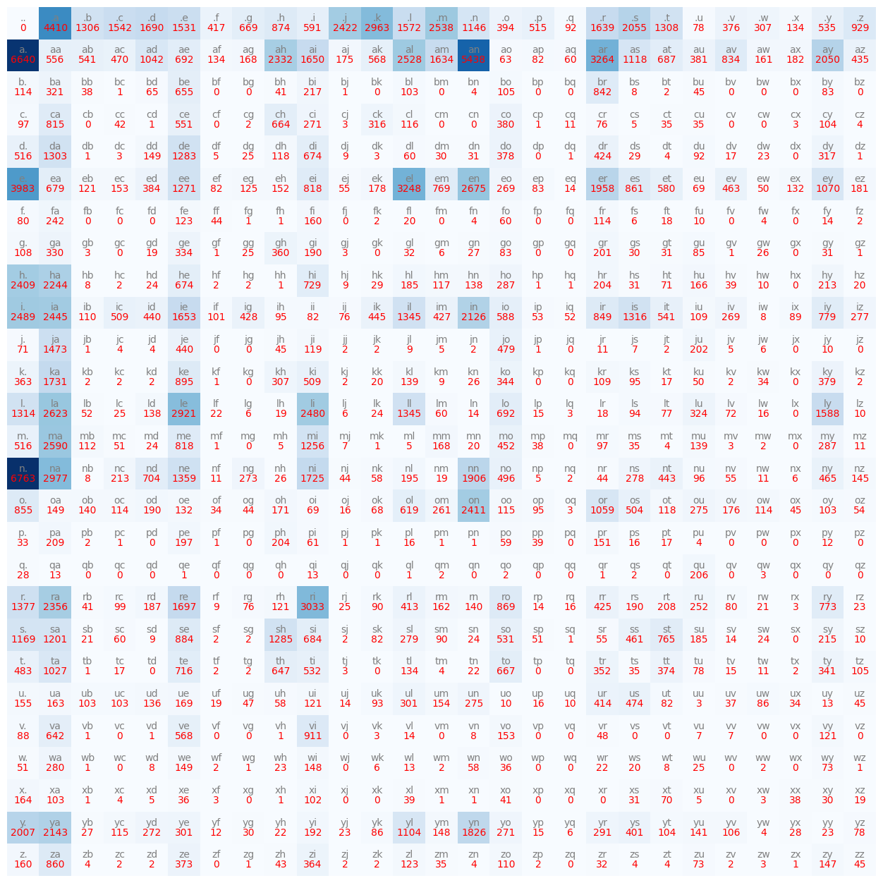

Every character pair now has a small but nonzero probability. The +1 is the strength of the smoothing: using +0.1 leads to lighter smoothing and +10 creates a uniform distribution.

This works well for the count-based model. But once you move to a neural network trained with gradient descent, there's no count matrix to add to. You need the same idea expressed in terms of the loss function.

L2 Regularisation (the Neural Network Equivalent)

In the neural network version, the model learns a weight matrix W. The raw predictions (logits) are logits = xenc @ W, where xenc is a one-hot encoded input character. Logits pass through softmax to become probabilities.

Without regularisation, the loss is just the negative log-likelihood:

xenc = F.one_hot(torch.tensor(xs), num_classes=27).float()
logits = xenc @ W
counts = logits.exp()
probs = counts / counts.sum(1, keepdim=True)

loss = -probs[torch.arange(len(xs)), ys].log().mean()

Adding L2 regularisation appends a penalty term:

loss = -probs[torch.arange(len(xs)), ys].log().mean() + 0.01*(W**2).mean()

Here is what each part does:

Mechanically: The penalty squares every weight in W, takes the average, and multiplies by a small constant (0.01). That value is added to the loss.

The competing pressure: Gradient descent minimises total loss, so the network now has two objectives in tension:

1. Make predictions accurate: minimise the negative log-likelihood.
2. Keep weights small: minimise 0.01*(W**2).mean().

Why large weights cause overfitting: Without the penalty, nothing stops the network from pushing weights to very large positive or negative values, making predicted probabilities approach absolute 1.0 or 0.0. The model becomes extremely confident about the training data — and generalises poorly to anything new.

The smoothing effect: By forcing weights towards zero, the logits (xenc @ W) also stay close to zero. Near-zero logits through softmax produce a nearly uniform distribution—about $1/27$ per character in a 27-character vocabulary. This is directly analogous to adding +1 to counts in Laplace smoothing: no transition gets assigned near-zero probability, and the 0.01 constant controls how strong that effect is.

L2 regularisation is the neural network's solution to the same problem that Laplace smoothing solved in the count-based model.

Types of Regularisation

L2 is the most common form, but there are others worth knowing.

L2 Regularisation (Ridge / Weight Decay)

The math: alpha*(W**2).mean()

The effect: Shrinks all weights towards zero, but rarely forces any to be exactly zero. Squaring amplifies large values, so the penalty hits large weights hard while being lenient on small ones. Weight importance gets distributed across many small values rather than concentrated in a few large ones.

When to use it: The default. When unsure, use L2.

L1 Regularisation (Lasso)

The math: alpha*(W.abs().mean())

The effect: Also shrinks weights towards zero, but actively forces many of them to become exactly zero. Because the penalty is linear rather than quadratic, a small weight is penalised proportionally just as harshly as a large one—the pull towards zero never weakens. The result is a sparse model where many weights are completely gone.

When to use it: When doing feature selection. If there are thousands of inputs (gene expressions, survey responses) and only a handful are actually predictive, L1 will zero out the useless ones, leaving a smaller and more interpretable model.

Elastic Net

The math: alpha*(W.abs().mean()) + beta*(W**2).mean()

The effect: A blend of L1 and L2. It encourages sparsity while maintaining the smooth behaviour of L2 when features are correlated. L1 alone can be erratic when two features are nearly identical — it arbitrarily zeros one and keeps the other. Elastic Net handles this more gracefully.

When to use it: When there are highly correlated inputs and want sparse outputs, but L1 alone is behaving unpredictably. The cost is two hyperparameters to tune (alpha and beta) instead of one.

How to Choose in Practice

1. Start with L2. In modern deep learning— Transformers, ResNets, LLMs—L2 weight decay is the default, often baked directly into the optimiser (see AdamW).
2. Switch to L1 if interpretability matters. When doing data science on tabular data and need to surface which variables actually drive the outcome, L1 will do that automatically.
3. Avoid L1 for embeddings. In language models, all embedding dimensions carry some fragment of meaning. L1's tendency to zero them out is a liability, not an asset. Stick with L2 combined with architectural regularisations like Dropout and Layer Normalisation.

Why L1 Creates Sparsity

The reason L1 pushes weights to exactly zero while L2 just makes them small is something I hadn't seen explained clearly before. It comes down to the shape of the penalty near zero.

The optimiser is minimising:

Total Loss = Prediction Error + Penalty

Why not everything goes to zero: If every weight became 0.0, the penalty would drop to zero, but the network would make random guesses for every prediction. The prediction error would be enormous, so the total loss would go up. Weights that are actually useful never get zeroed out.

The per-weight trade-off: For every weight, the network is implicitly asking: "Does keeping this weight reduce my prediction error by more than the penalty costs me?"

• Useful weight (e.g., the one connecting q to u): removing it spikes the prediction error. The network pays the penalty to keep it.
• Useless weight (e.g., the one connecting q to x): it barely affects accuracy either way. The network concludes this weight isn't earning its keep and drops it to 0.0.

Why L1 reaches zero but L2 doesn't:

With L2, the penalty is proportional to the square of the weight. As the weight shrinks, the penalty shrinks quadratically—a weight of 0.001 carries a penalty of only 0.000001. The pressure to keep shrinking nearly disappears, so L2 never quite reaches absolute zero.

With L1, the penalty is proportional to the absolute value. A weight of 0.001 still carries a penalty of 0.001. The pull towards zero never weakens, no matter how small the weight gets. Useless weights get dragged all the way to exactly 0.0; useful ones settle at an equilibrium where the prediction accuracy they provide outweighs the penalty.

That asymmetry—linear vs. quadratic penalty near zero—is the entire reason L1 produces sparse models and L2 doesn't.