Receptive Fields in CNNs: Why Depth Beats Big Kernels

• What Is a Receptive Field?
• How the Receptive Field Grows With Depth
• Generalising to Stride and Pooling
• Why Depth Beats a Single Large Kernel
• The Effective Receptive Field
• Conclusion
• Resources

The first part, CNN Fundamentals: Kernels, Convolution, and Feature Maps, of this series covered how a single convolutional layer turns an input into a feature map, and noted that a CNN's feature vector at any given location only has access to a small local neighbourhood — its receptive field — rather than the whole image. This post is about that neighbourhood: how it's defined, how it grows as a network gets deeper, and why that growth is the real reason CNN architectures favour many small filters over a few large ones.

What Is a Receptive Field?

The receptive field of a given neuron (equivalently, a given spatial location in a feature map) is the region of the original input image that can influence that neuron's value.

This follows directly from how convolution works: a single 3×3 filter only ever reads a 3×3 patch of whatever it's fed. So a neuron in the first convolutional layer of a network has, by definition, a 3×3 receptive field on the input image — it simply has no way to "see" anything outside that patch.

How the Receptive Field Grows With Depth

The receptive field grows as you stack layers, even though each individual layer's kernel stays small. Consider a neuron in the second convolutional layer: it looks at a 3×3 patch of the first layer's output feature map. But each of those 9 positions in that patch was itself computed from a 3×3 patch of the original image, and those 9 source patches overlap and collectively span a larger area than 3×3. So the second-layer neuron indirectly depends on a bigger region of the original input than its own kernel size would suggest.

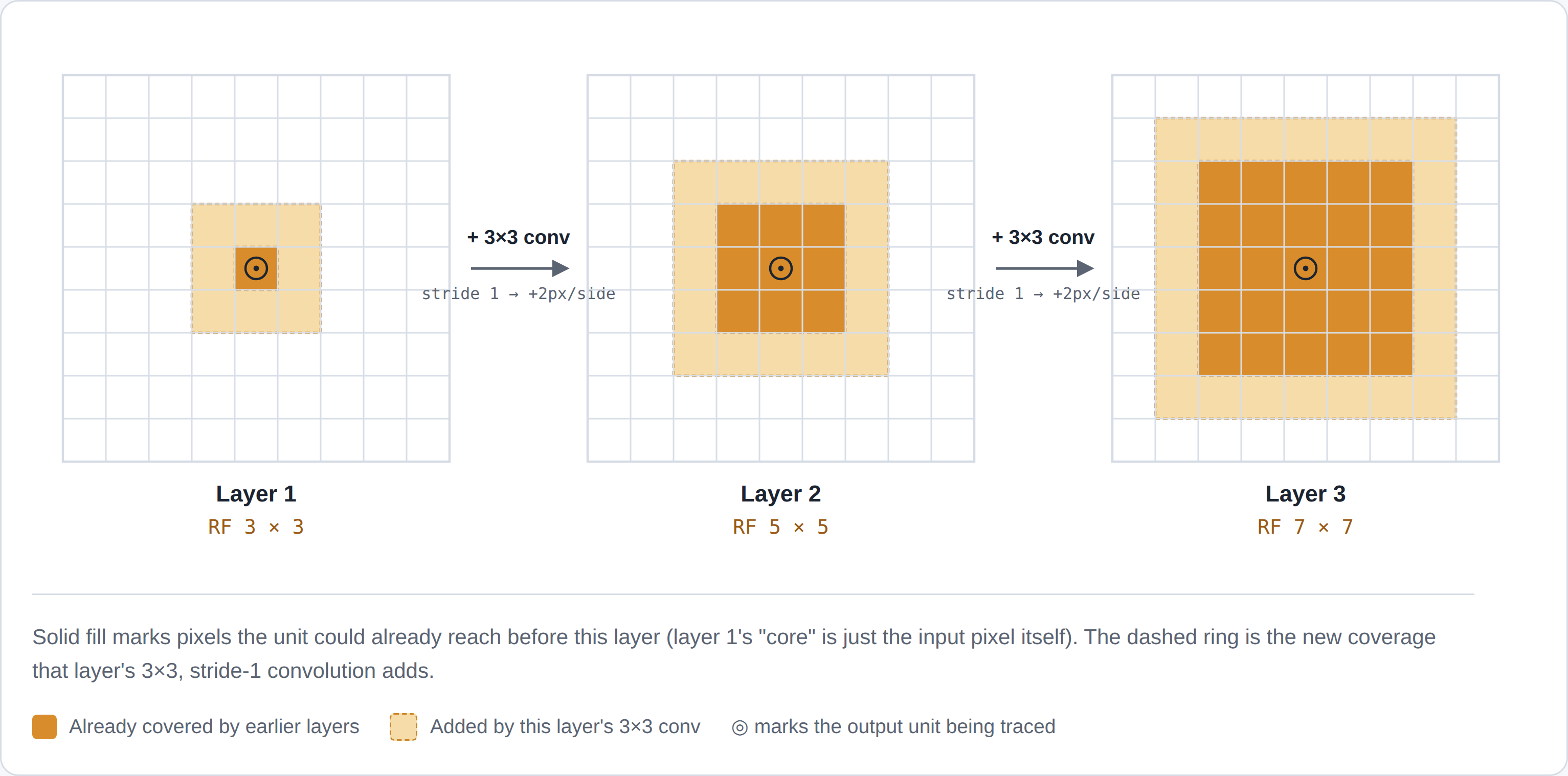
For stacked k×k kernels with stride 1, this generalises to a simple recurrence: each layer adds k − 1 pixels to the receptive field.

$\text{RF}_l = \text{RF}_{l-1} + (k-1)$

For 3×3 kernels, that's +2 pixels per layer: layer 1 → 3×3, layer 2 → 5×5, layer 3 → 7×7, and so on — exactly what the diagram shows. This is why deep CNNs can recognise large-scale structure (a whole face, a car) using only small 3×3 filters throughout: depth compounds the effective field of view, without ever needing a physically large kernel.

Generalising to Stride and Pooling

The formula above assumes stride 1 everywhere, which isn't always true — pooling layers in particular are usually stride 2. The general version tracks a second quantity alongside the receptive field: the jump (sometimes called the stride product — terminology borrowed from Araujo et al.'s treatment of the topic), which is how many input pixels apart two adjacent output positions are.

$\text{jump}_l = \text{jump}_{l-1} \times s_l \qquad \text{RF}_l = \text{RF}_{l-1} + (k_l - 1) \times \text{jump}_{l-1}$

where jump_0 = 1 (adjacent pixels in the raw input are, trivially, 1 pixel apart). With every layer at stride 1, jump stays at 1 and this collapses back to the simpler formula above. But a stride-2 layer — a 2×2 max-pool, for instance — doubles the jump, which means every layer after it adds receptive field twice as fast per unit of kernel size. Concretely: a 3×3, stride-1 conv (RF 3, jump 1) followed by a 2×2, stride-2 max-pool (RF 3 + (2−1)×1 = 4, jump 2) followed by another 3×3, stride-1 conv (RF 4 + (3−1)×2 = 8, jump 2) reaches an 8×8 receptive field in three layers — pooling is a cheap way to grow the receptive field quickly, which is part of why it shows up so often between convolutional blocks.

Why Depth Beats a Single Large Kernel

Receptive field size is one reason CNN architectures go deep with small filters, rather than using one layer with a giant kernel to cover the same area directly. Compare a single 7×7 kernel against three stacked 3×3 layers, both of which produce a 7×7 receptive field:

• A 7×7 kernel has 7×7 = 49 weights per input channel.
• Three stacked 3×3 layers have 3×(3×3) = 27 weights per channel in total — nearly half as many.

The stacked version is also cheaper in FLOPs for the same reason, and it inserts two extra nonlinearities (e.g. ReLU) between the three convolutions instead of the single one the 7×7 kernel would apply. Each nonlinearity lets the network learn a more complex, non-linear function of the input rather than a single linear projection, so the stacked layers reach the same receptive field with fewer parameters and more representational flexibility. This is precisely the argument Simonyan and Zisserman made for VGGNet's design (stacking small 3×3 convolutions instead of using the larger 11×11/7×7 kernels earlier architectures like AlexNet used), and it's been the default assumption in CNN design since.

The Effective Receptive Field

The formulas above describe the theoretical receptive field — the full region of the input that could, in principle, affect a given neuron's output. In practice, not every pixel in that region matters equally.

Luo et al. (2016) showed that a neuron's actual sensitivity to pixels within its theoretical receptive field isn't uniform — it's concentrated near the centre and falls off, roughly like a Gaussian, towards the edges. Pixels near the centre are on the path of many more of the intermediate computations (they're reachable through many more of the overlapping patches at each layer) than pixels near the edge, which are only reachable through one narrow chain of positions. The practical consequence is that the effective receptive field — the region that meaningfully influences the output — is smaller than the theoretical one, and grows proportionally to the square root of the network's depth rather than linearly with it. This doesn't invalidate the arithmetic above (the theoretical receptive field is still the hard upper bound on what could matter), but it's a reason architectures often use techniques like dilated convolutions or attention to grow the effective — not just theoretical — field of view.

Conclusion

The receptive field is what makes CNNs work at all despite each filter only ever looking at a tiny local patch: stacking layers grows a neuron's effective view of the input geometrically cheap in parameters, geometrically rich in nonlinearity, and — per the effective receptive field result — still concentrated where it matters most, near the centre. Combined with CNN Fundamentals: Kernels, Convolution, and Feature Maps's account of how a single convolutional layer computes its output, this is most of the intuition needed to read a CNN architecture diagram and understand why it's shaped the way it is.

Resources

• Luo, W., Li, Y., Urtasun, R., & Zemel, R. (2016). Understanding the Effective Receptive Field in Deep Convolutional Neural Networks. Advances in Neural Information Processing Systems (NeurIPS) 29.
• Simonyan, K., & Zisserman, A. (2014). Very Deep Convolutional Networks for Large-Scale Image Recognition. arXiv:1409.1556.
• Araujo, A., Norris, W., & Sim, J. (2019). Computing Receptive Fields of Convolutional Neural Networks. Distill.